
02: Lidar perception: PointNet, VoxelNet, and CenterPoint
Published:
Lidar provides measured points on visible surfaces. Unlike pixels, these samples already carry three-dimensional positions, but they do not form a regular image: their number varies, their spacing is uneven, and their order has no physical meaning. The central design problem is how to turn that set into a representation a network can process efficiently.
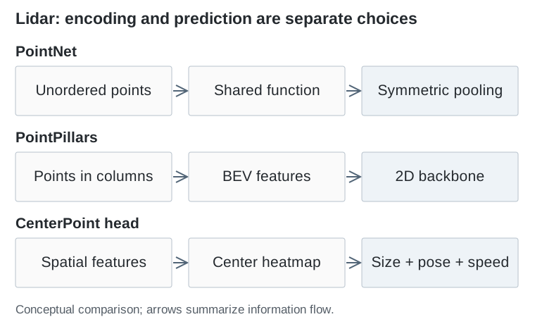
The progression from PointNet to CenterPoint changes two separate things: how evidence is encoded and how objects are parameterized. Keeping those decisions separate makes the literature much easier to read.
PointNet: learn directly from an unordered set
PointNet — Qi et al., CVPR 2017 applies a shared function to each point, then combines the resulting features with a symmetric operation such as maximum pooling. Reordering the input points therefore does not change the pooled representation.
In compact form, a set feature is g = max_i φ(p_i): p_i is a point, φ is the same learned transformation for every point, and the maximum is taken separately for each feature channel. Classification uses the global feature; segmentation can combine it with individual point features.
The strength is that no artificial point ordering is needed. The limitation is that one global aggregation is a weak way to describe local shape. PointNet++ — Qi et al., NeurIPS 2017 adds hierarchical neighborhood grouping and feature extraction. These papers supply important building blocks, rather than a complete recipe for driving detection by themselves.
VoxelNet and SECOND: introduce a spatial grid
VoxelNet — Zhou and Tuzel, CVPR 2018 divides space into small 3D cells called voxels. A learned encoder aggregates the points within each occupied cell; later layers combine information across cells and predict objects.
This restores spatial neighborhoods: nearby array locations correspond to nearby physical locations. The price is the grid itself. Halving cell size in all three dimensions increases the possible number of cells eightfold for the same volume.
SECOND — Yan et al., Sensors 2018 uses sparse convolution to make this representation more practical. The computation tracks active spatial locations rather than allocating equivalent work to every empty voxel. Sparse processing reduces wasted work, although runtime still depends on occupancy, feature size, and the implementation.
PointPillars: compress height before the main backbone
PointPillars — Lang et al., CVPR 2019 groups points into vertical columns. A learned encoder summarizes each column, and the features are scattered into a bird’s-eye-view, or BEV, grid. A 2D convolutional network then performs the main spatial processing.
The points can still carry height inside the pillar encoder. What disappears is an explicit stack of height cells in the main backbone. This is a deliberate compression: a road scene often benefits greatly from horizontal layout, while a full 3D feature volume is expensive.
The tradeoff becomes visible around vertically complicated structures. A representation that combines an overpass and the road beneath it must preserve their distinction in feature channels rather than separate grid layers.
CenterPoint: change the object representation
CenterPoint — Yin et al., CVPR 2021 predicts object centers on a BEV heatmap, together with properties such as size, height, orientation, and velocity. Further refinement can use features associated with the predicted object.
A center is a compact target even when the object’s orientation changes. CenterPoint also uses estimated motion for a simple tracking procedure. Its contribution is therefore different from the voxel-to-pillar change: center-based prediction is a detection-head decision and can be paired with different feature encoders.
| Choice | What it changes | Main cost or limitation |
|---|---|---|
| Point neighborhoods | How local geometry is gathered | Neighborhood search and irregular processing |
| Voxels | How 3D space is indexed | Resolution and active-cell count |
| Pillars | Where height is compressed | Less explicit vertical structure |
| Center-based detection | How objects are predicted | Still depends on the encoded evidence |
Why this family matters beyond lidar
BEV became a useful meeting place for driving tasks because distance and direction have consistent physical meaning there. A displacement of one meter is one meter regardless of which camera sees it.
Lidar makes the initial placement relatively direct: measured points can be transformed into the vehicle’s coordinate frame. Camera-only methods face a harder version of the same problem because they must infer depth. Their subsequent use of BEV should be understood as borrowing a useful spatial interface, rather than making camera measurements equivalent to lidar.